JBrowse2¶

Overview¶

This section will provide some quick training on how to use JBrowse2. You can also learn more via the JBrowse2 User Guide.

With the switch to JBrowse2, we have decided that not all the genomes will get migrated to JBrowse2 and that going forward, we will focus on a select number of genomes from each crop (the genomes everyone use as references or are genetically diverse) and provide value-added analyses to these genomes that will facilitate genomic discovery. We will adjust the genomes available in JBrowse2 to fit the community needs.

Advantages of using JBrowse2 versus JBrowse1

Can view multiple genome chromosomes/scaffolds in one panel

Can view multiple genomes in same session

Can view synteny analysis results and relationships between genomes

Can generate dot plots between two genomes that can be used to navigate to genome regions

Can view pangenome data

Same features in JBrowse2 as JBrowse1

Can view annotated genes and mRNA for genome and can zoom to nucleotide level

Can view aligned PCR-based markers and SNP markers and QTL

Can search by gene, mRNA, marker, or trait names

Accessing JBrowse2¶

JBrowse2 can be accessed by clicking on the genome name for the respective genome on the JBrowse page.

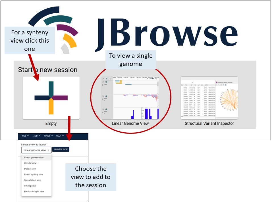
If you are started with an empty session, click on ‘Linear Genome View’ and select a genome of interest.

Navigating JBrowse2¶

When adding a genome, you can select a specific chromosome/scaffold or show all regions of the assembly.

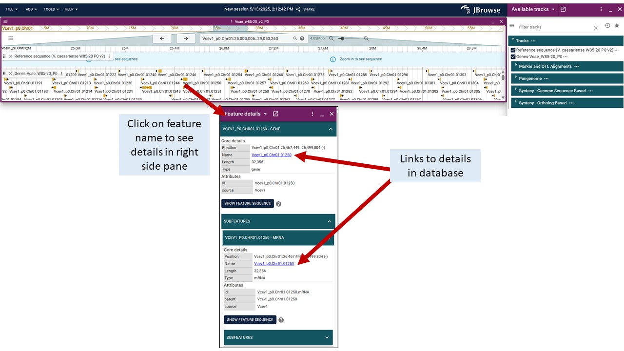
To turn on/off data tracks, either click the ‘open track selector’ button or click the hambuger menu in the upper left of genome track. Once the track selector is open, you can click the boxes next to the track names to turn tracks on/off. Click on the section headers to expand the sections and see the additional tracks.

To view details about features, click on the feature and a ‘Feature details’ pane will open up on the right side of the screen (over the track selector section). Blue hyperlinks on feature names or dbxref take you to more details on GDV.

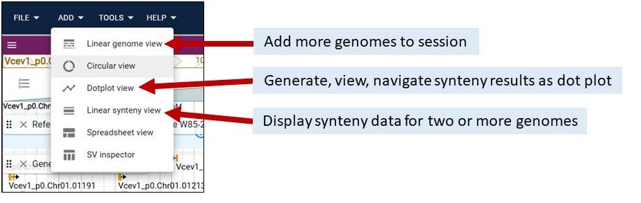
In JBrowse2, you can add multiple genome tracks or other data type tracks in the same session. Click on ‘Add’ and select the track type. See below for details about the Linear Synteny View and Dotplot View.

Linear Synteny View¶

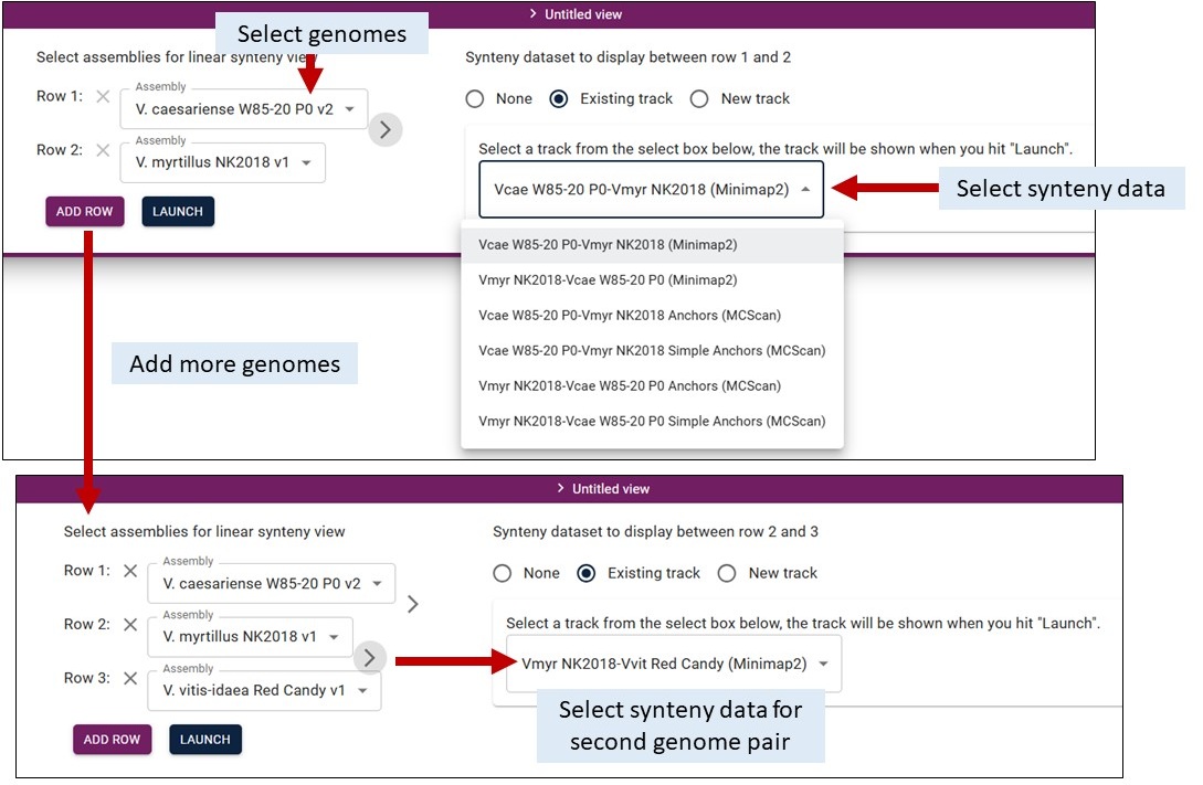
Once you have selected the Linear Synteny View, you get an interface to select two or more genomes and the synteny data track to display. We provide pairwise comparisons computed by Minimap2 (uses genome sequences) and MCScan (uses mRNA sequences). Selecting which data to display is similar. Viewing the results from each tool is detailed below. Clicking on the features displays more information, just like for the other tracks.

By default, you need to select at least two genomes from the dropdown menus in Row 1 and Row 2. You then select the synteny data to display from another dropdown menu on the right. You can add more pairwise comparisons by clicking ‘Add Row’, selecting the genomes, and then click on the arrow between the pairs to select the synteny dataset.

This is an example of synteny data from Minimap2 and what all the colors mean. The genomes are displayed with the linking synteny track in the middle. You can turn on tracks, including the synteny data track, in the track selector. Here are what the colors mean for the synteny track in the middle of the genomes.

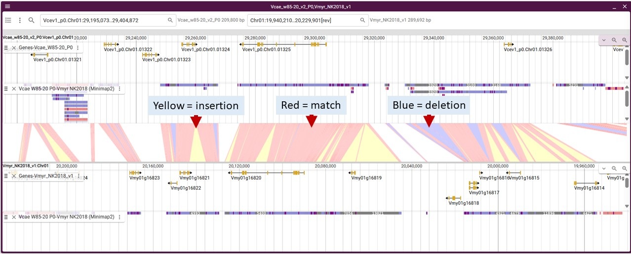
Within the Minimap2 tracks, here are what the colors mean on the syntenic blocks.

For MCScan, you will see two tracks for each genome pair: Simple Anchors and Anchors. The Anchors track will display the syntenic genes (really the mRNA) between the genomes which means the tracks is a collection of many features. The Simple Anchors track was generated from the Anchors track and displays larger syntenic blocks which simplifies the display a bit.

When you zoom in, you will see the individual syntenic blocks. In this example, the center synteny track is the Simple Anchors and we have turned on the Simple Anchor and Anchor tracks for each genome.

In this image, we have used the Anchors track for the center track and turned on the Anchors track and gene track for each genome. If you hover over the features in the Anchors tracks it will display the orthologous gene names from each genome.

Dotplot View¶

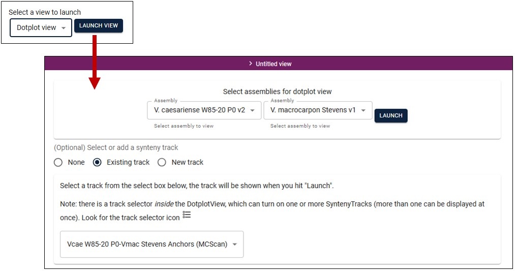
You can also view the synteny data in a dotplot. Once you select the Dotplot View, you select two genomes and the dataset to use, similar to the Linear Synteny View.

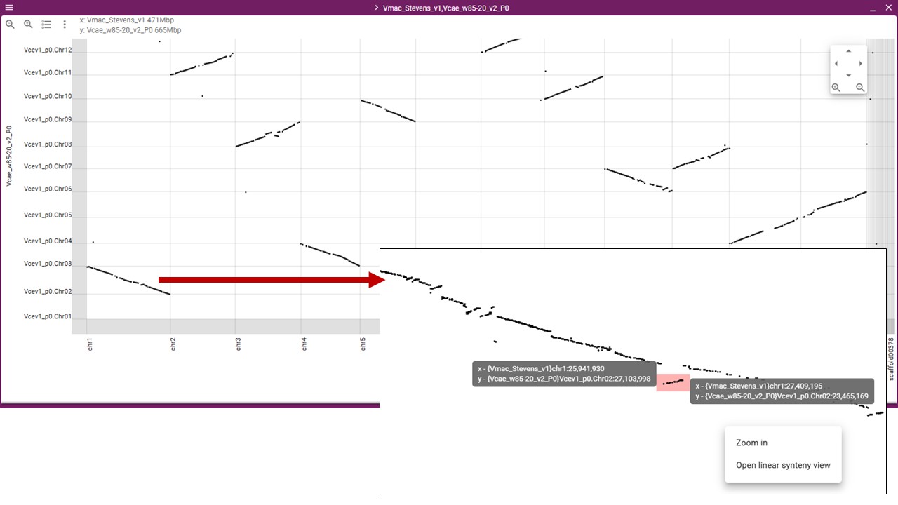
You will then see the dotplot and can gighlight regions to zoom in on and also have the option to display that highlighted region in a Linear Synteny View.

Pangenome Data¶

Pangenome data was parsed in relation to the reference genomes that are in JBrowse2 and the pangenome analysis. The pangenome data is available as tracks in the Track Selector under the ‘Pangenome’ section. The reference genome will be a gray bar and the differences between the reference and the other genomes are noted. The base differences are indicated as well as insertions and regions without matches. Insertions less than 10 bases are noted by a purple bracket. Insertions over 10 bases are a purple bar with the number of bases noted.